


All Issues
Modeling guides groundwater management in a basin with river–aquifer interactions
Publication Information
California Agriculture 72(1):84-95. https://doi.org/10.3733/ca.2018a0011
Published online March 13, 2018
NALT Keywords
Abstract
The Sustainable Groundwater Management Act (SGMA) of 2014 seeks to maintain groundwater discharge to streams to support environmental goals. In Scott Valley, in Siskiyou County, the Scott River and its tributaries are an important salmonid spawning habitat, and about 10% of average annual Scott River stream flow comes from groundwater. The local groundwater advisory committee is developing groundwater management alternatives that would increase summer and early fall stream flows. We developed a model to provide a framework to evaluate those alternatives. We first created a water budget for the Scott Valley groundwater basin and integrated the detailed, spatiotemporally distributed water budget results into a computer model of the basin that simultaneously accounted for groundwater flow, stream flow and landscape water fluxes. Different conceptual representations (using the MODFLOW RIV package and MODFLOW SFR package) of the stream–aquifer boundary provided significantly different results in the seasonal dynamics of groundwater–surface water fluxes. As groundwater sustainability agencies draw up plans to meet SGMA requirements, they must choose and test simulation tools carefully.
Full text
Management of California's water supplies serves diverse goals. Securing the needs of urban and agricultural water customers is a key goal. Meeting environmental health, ecosystem services and stream water quality goals has also been an integral part of many California water management systems. To meet this range of goals, groundwater, soil water and surface water will need to be managed conjunctively, management will likely become more tightly linked with land use and land resources planning and management, and modelling will play a key role in the development of successful and useful management plans.
The 2014 California Sustainable Groundwater Management Act (SGMA) and recent salt- and nitrate-related regulations to protect groundwater quality have put a focus on groundwater resources management, both quality and quantity, particularly in agricultural regions (Harter 2015). They mandate that local agencies pursue groundwater sustainability goals: avoiding long-term groundwater storage depletion, land subsidence, seawater intrusion, groundwater management–related water quality degradation, and deterioration of groundwater–surface water interactions.
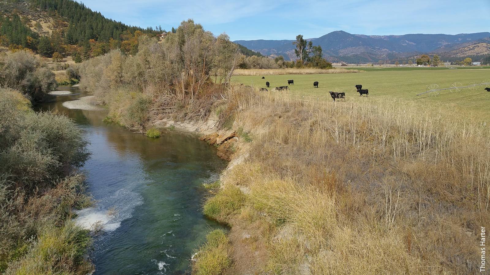
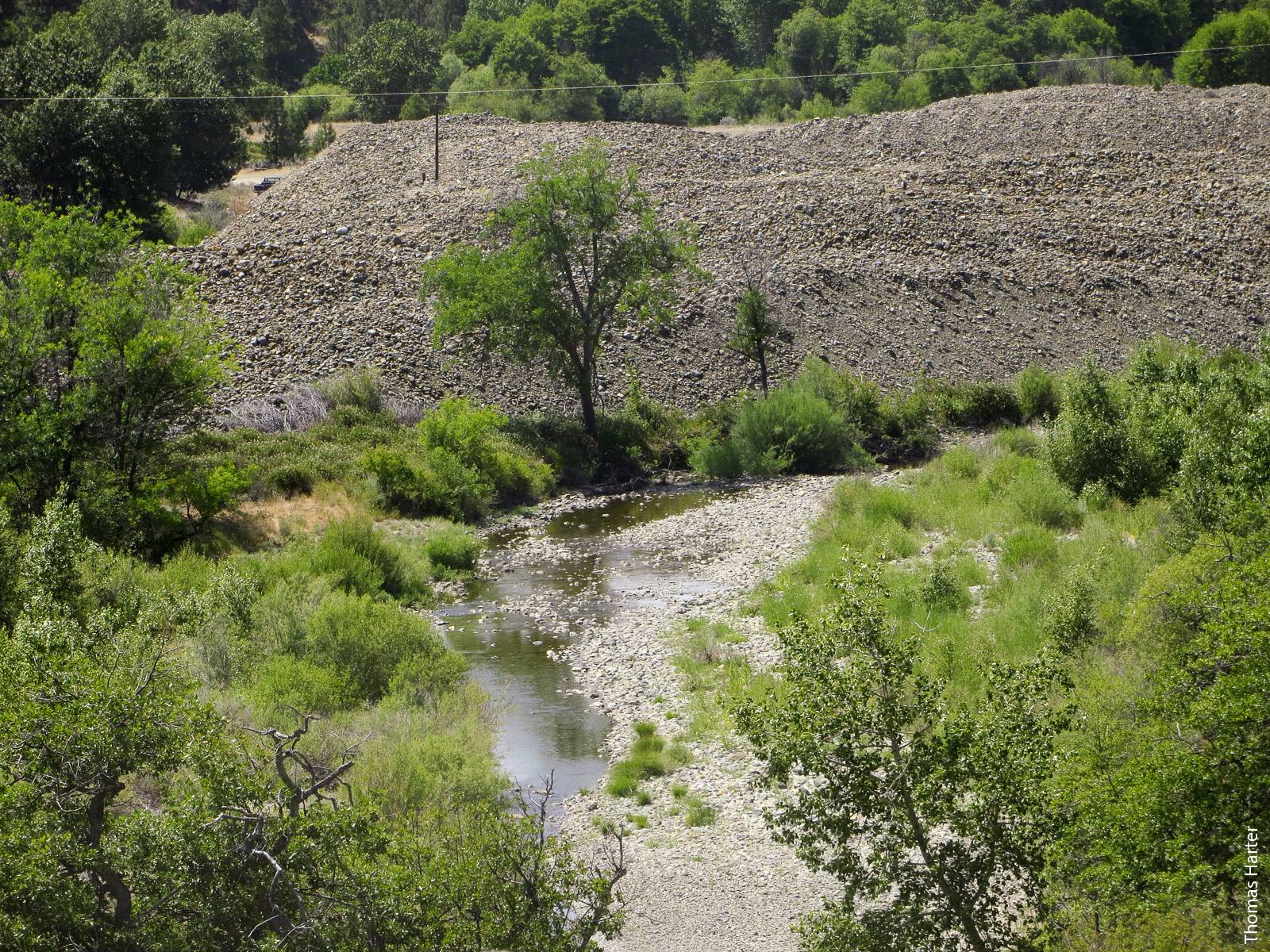
The Scott River is an important salmonid spawning habitat that depends on groundwater to maintain stream flow during the summer. A hydrologic model developed by UC researchers can help predict the impact of different groundwater and surface water management scenarios on stream flow.
Particularly important under the SGMA regulations is the interaction between groundwater and surface water: how do groundwater management decisions — by individual landowners or by groundwater sustainability agencies (GSAs) — impact not only beneficial users, but also streams (Zume and Tarhule 2011) and ground-water-dependent ecosystems (GDEs) (Boulton and Hancock 2006; Hatton 1998). Prominent California examples of areas where groundwater–surface water interactions are already addressed include the Napa River in Napa County and the Scott River in Siskiyou County. Both feature important salmonid fish habitat and therefore temperature is a critical issue (Brown et al. 1994; Moyle and Israel 2005); and low or decreased late-summer stream flow over the last half-century has impacted the quantity and quality of fish habitat (Kim and Jain 2010; NCRWQCB 2005; Nehlsen et al. 1991). During drought, portions of these rivers may temporarily dry up. In intermontane Scott Valley, dry sections disconnect lower sections of the stream from tributaries in the headwaters. Summer stream temperatures in the Scott River are affected by groundwater discharge into the streambed and by riparian shading and were being addressed under the federal Clean Water Act (NCRWQCB 2005) before SGMA.
Some measurements can be collected in the field to evaluate groundwater–surface water interactions, but computer models are needed to fully understand groundwater basin flow dynamics and assess impacts to stream flow under future groundwater management scenarios. For example, computer models can show the response of integrated water systems to management decisions such as pumping and intentional recharge. They are expected to play a key role in the implementation of SGMA and regulatory efforts.
Various modeling approaches have been developed for groundwater–surface water interactions (Furman 2008; Harter and Seytoux 2013). These range from analytical or spreadsheet tools (Foglia, McNally, Harter 2013) and coupled or iteratively coupled numerical model codes for computer simulations, such as the MODFLOW river (RIV) package (Harbaugh et al. 2000) and the MODFLOW stream flow routing SFR1 package (Prudic et al. 2004) and SFR2 package (Harbaugh 2005; Niswonger and Prudic 2005), to fully coupled models such as ParFlow (Ashby and Falgout 1996; Kollet and Maxwell 2006) and Hydrogeosphere (Brunner and Simmons 2012).
Fully coupled models provide the physically and mathematically most consistent and complete integration of groundwater, surface water and soil water systems. But they are computationally more expensive and require more parameterization (data input) than iteratively coupled models. In coupled or iteratively coupled models, multiple models are coupled such that one model provides input to the other model and vice versa, sometimes iteratively. Full coupling may not always yield better results (Furman 2008). For some applications, statistical models or analytical tools, which are based on highly simplified concepts and therefore have the least data input requirements and are computationally much less demanding, may be appropriate.
In Scott Valley, groundwater–surface water interactions are analyzed as part of an action plan to meet temperature TMDL (Total Maximum Daily Load) requirements for the Scott River. Climate change and groundwater pumping for irrigation in the valley have impacted late-summer and early fall stream flows in the Scott River (Drake et al. 2000). The local groundwater advisory committee is developing potential groundwater management scenarios that would increase summer and early fall stream flows. To evaluate those scenarios, we explored three levels of conceptual complexity at which information can be obtained about groundwater–surface water interactions: a water budget approach, a groundwater model with a conceptually simplified stream model (RIV) and a fully coupled groundwater–surface water model (SFR).
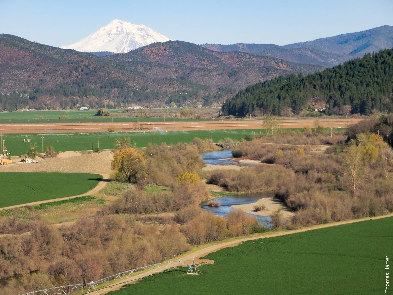
Almost 70% of Scott Valley is used for agricultural production, with a nearly even split between alfalfa/grain and pasture.
Scott Valley study area
Our study area was Scott Valley in northern California. Almost 70% of the valley is used for agricultural production, with a nearly even split between alfalfa/grain and pasture.
Geography and climate
Scott Valley is an intermontane 220-square-kilometer agricultural groundwater basin at an elevation of 2,600 to 3,100 feet in Siskiyou County (fig. 1). The Scott River flows from south to north along the east-central and northern portion of the valley. At the valley's northwest corner, the river descends into a gorge before joining the Klamath River several miles below Scott Valley. The Scott River watershed above Scott Valley extends into the surrounding Klamath Mountains to elevations of over 8,500 feet. The river and its tributaries are an important salmonid spawning habitat, home to native populations of the threatened Oncorhynchus kisutch (coho).
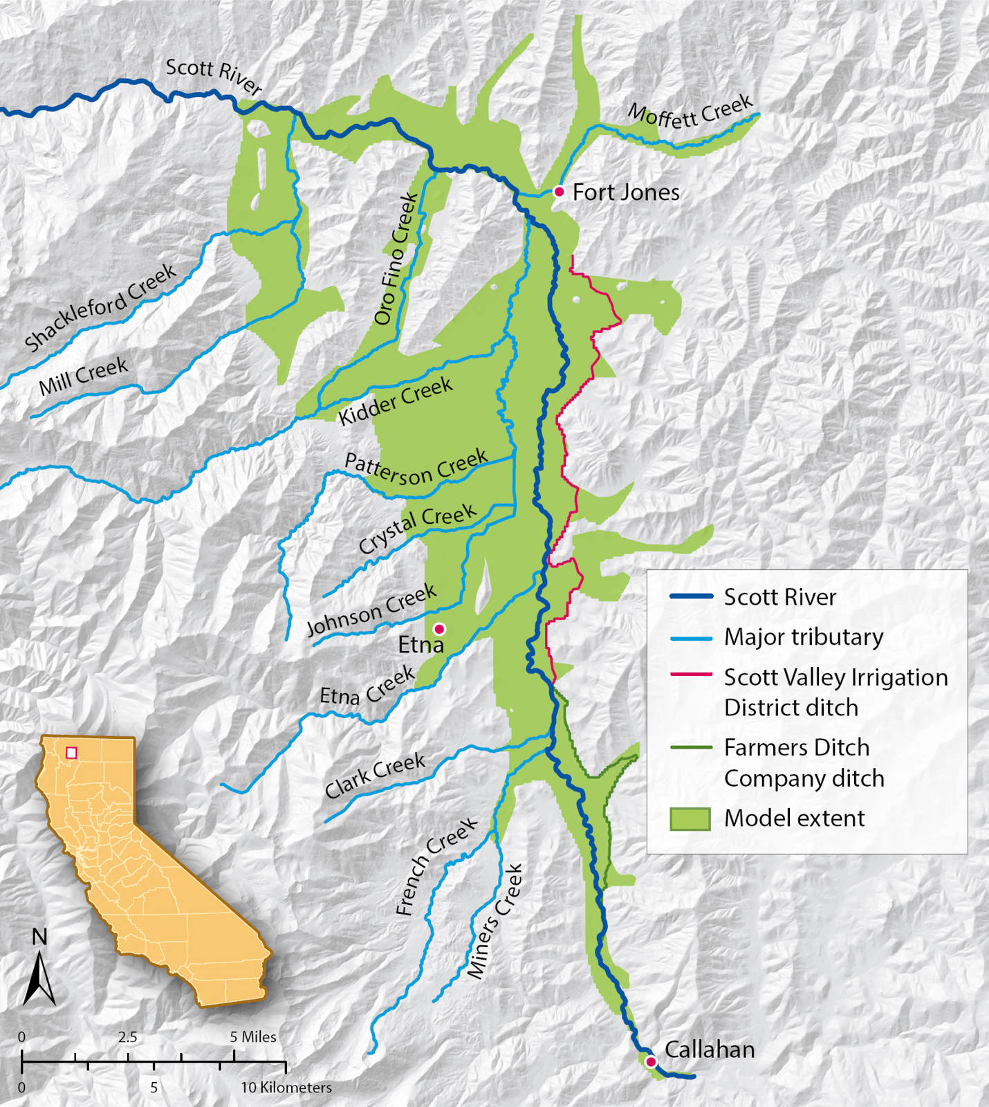
FIG. 1. The boundaries of the groundwater model study in Scott Valley, and its surface waters. The Scott River and its tributaries are an important salmonid spawning habitat, home to native populations of the threatened coho. Source: Model extent derived from Mack (1958) and Soil Survey Geographic Database (SSURGO) data. Projection: North American Datum 1983, UTM Zone 10.
Scott Valley formed primarily due to movement along an eastward dipping normal fault, with unconsolidated, highly heterogeneous fluvial and alluvial fan deposits forming an alluvial groundwater basin (Mack 1958). Surrounding the valley, the geology is comprised of relatively impermeable bedrock composed of metamorphic and volcanic units, although fractures do yield some water in the form of springs at the margins of the valley and in surrounding upland areas.
Aquifer thickness may be as much as 400 feet in the wide central part of the valley (Mack 1958). However, there is no evidence of sufficiently coarse material to support agricultural groundwater pumping below 250 feet (Foglia, McNally, Harter 2013). The aquifer pinches out at the valley margin.
Climate in the valley is Mediterranean, with 89% of the nearly 500-millimeter average annual precipitation falling between October and April. Daily mean temperatures range from 70°F in July to 32°F in January. Precipitation depths in the surrounding mountains are much higher, and snowmelt is a major source for ephemeral tributaries feeding the Scott River and recharging into the aquifer. Snowmelt dominates Scott River flows through June. During the summer months, flows in the Scott River immediately below the montane valley (USGS gage 11519500 Ft. Jones) can drop to 4 cubic feet per second (cfs), while maximum flows during winter can reach 40,000 cfs. After snowpack storage has been depleted, the Scott River is dependent on discharge from the Scott Valley aquifer to support base flow. In dry years, sections of the Scott River overlying the valley floor become ephemeral.
Land use and irrigation
Land use was surveyed in 2000 (DWR 2000) and further refined using aerial photo analysis and on-the-ground verification through interviews with landowners. A total of 2,119 land use parcels overlie the Scott Valley groundwater basin (fig. 2): 710 parcels (17,400 acres) are alfalfa/grain (an 8-year rotation with, on average, 1 year of grain crop followed by 7 years of alfalfa), 541 parcels (16,600 acres) are pasture, 451 parcels (20,400 acres) belong to land use categories with significant evapotranspiration but no irrigation (e.g., cemeteries, lawns, natural vegetation) and 417 parcels (1,700 acres) represent land uses with no evapotranspiration or irrigation (e.g., residential areas, parking lots, roads, and — most significantly — historic mine tailings).
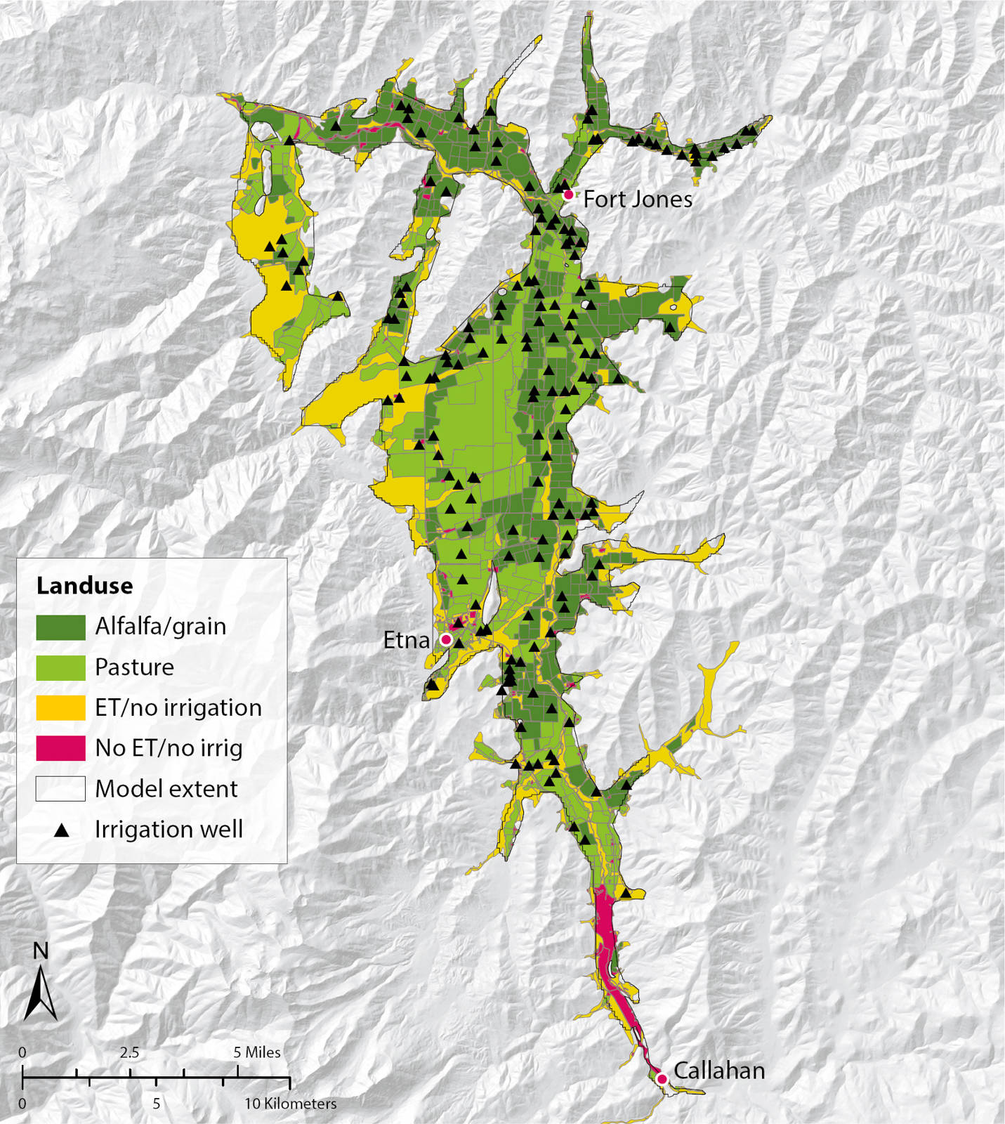
FIG. 2. Land use information and well locations in Scott Valley. ET/no irrigation reflects nonirrigated vegetation, e.g., lawns and riparian vegetation. No ET/no irrigation represents nonvegetated land surfaces including the mine tailings near Callahan. Well location information was obtained from well logs filed with the Department of Water Resources and verified in the field. Source: Model extent derived from Mack (1958) and SSURGO data. Land use polygon data source: DWR (2000). Revised to reflect 2011 land use patterns (GWAC, Groundwater Advisory Committee). Projection: North American Datum 1983, UTM Zone 10.
The year 2000 land use survey by DWR (DWR 2000) also identified the irrigation type associated with each land parcel. About 6,200 acres of cropland were identified as nonirrigated, dry or subirrigated. In Scott Valley, flood, center-pivot sprinkler and wheel-line sprinkler irrigation are used almost exclusively. Over the past 25 years, significant conversion from wheel-line sprinkler (but also from flood irrigation) to center-pivot sprinkler has occurred. For our study, we mapped the location (extent) and year of such irrigation-type conversions to land parcels by reviewing 1990 to 2011 aerial photos.
The beginning of the irrigation season is determined by soil moisture depletion but also by grower peer behavior. Earliest irrigation dates reported by local growers were March 15, March 24 and April 15 for grains, alfalfa and pasture, respectively. Growers irrigate based on soil moisture data, experience, peer behavior and established irrigation practices. The irrigation season typically ends on July 10, Sept. 1 and Oct. 15 for grain, alfalfa and pasture, respectively.
Water sources (identified for each land parcel by the DWR 2000 land use survey and updated through landowner survey) include groundwater, surface water, subirrigated (shallow groundwater table, not actually irrigated), mixed groundwater–surface water, and nonirrigated (dryland farming). Land parcels are distributed across nine subwatersheds associated with the major tributaries and the main stem Scott River. Discharge on these streams into the Scott Valley defines available maximum diversion rates for surface water irrigations. Where surface water is the only source of irrigation, lack of surface water will terminate the irrigation season. Groundwater pumping for a land parcel is from nearby or on-site irrigation wells. Well locations and type for the study area were obtained from DWR well permit records (fig. 2).
Hydrogeology
Within the alluvial groundwater basin of the Scott Valley, Mack (1958) distinguished six subareas (fig. 3). In our work, we also included the mine tailings at the southern end of the alluvial basin, an important hydrogeologic area consisting almost exclusively of reworked boulders from mine dredging operations (Foglia, McNally, Harter 2013).
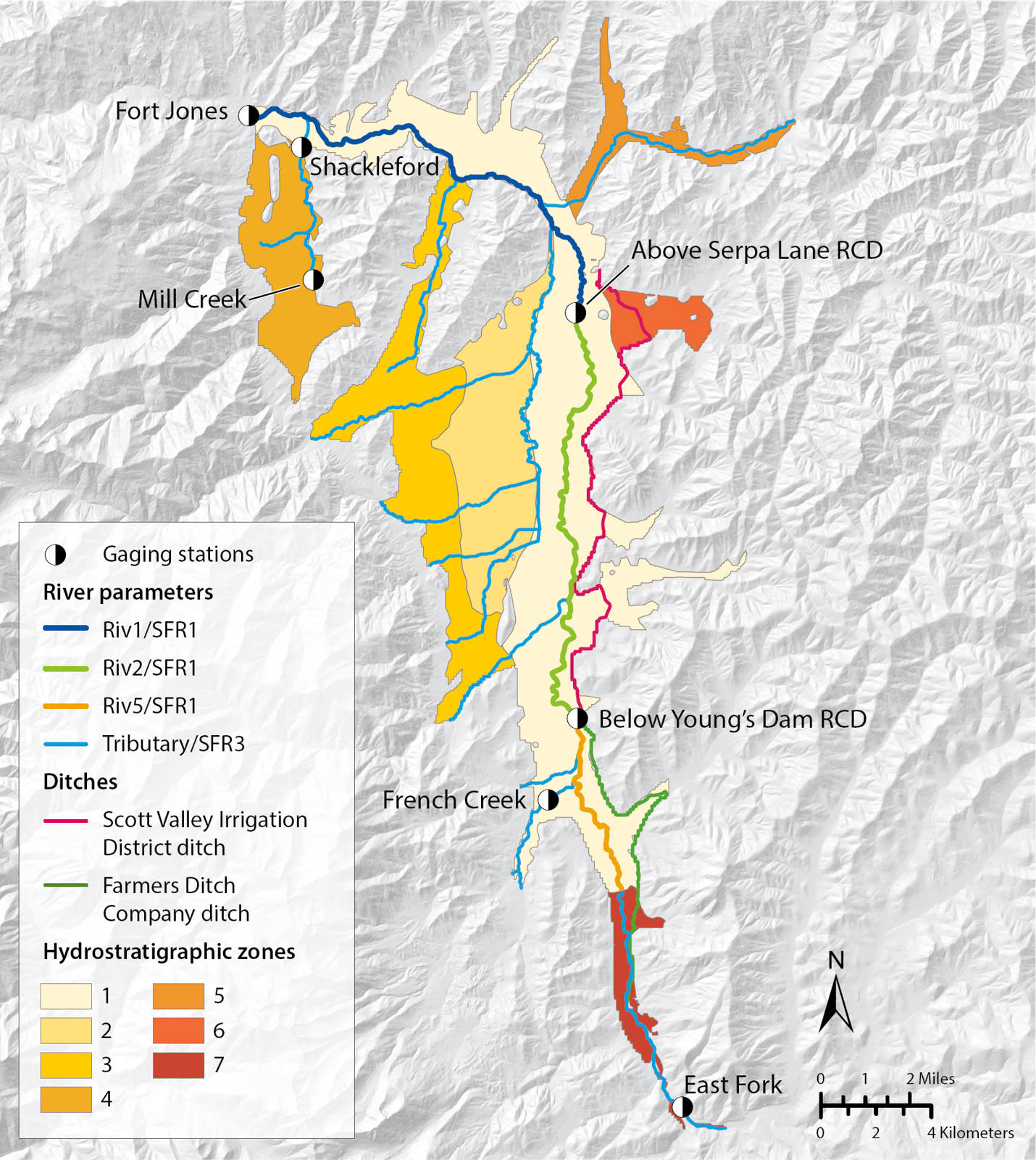
FIG. 3. Representation of the main characteristic of the modelled area, including boundary conditions, hydraulic conductivity and specific storage as defined by hydrostratigraphic zone, irrigation ditches, stream flow gaging stations and river segments (represented as Riv1, Riv2 and Riv5). Source: Model extent derived from Mack (1958) and Soil Survey Geographic Database (SSURGO) data. Projection: North American Datum 1983, UTM Zone 10.
Aquifer pumping tests were performed to determine hydraulic properties in the main subarea of the valley, along the Scott River corridor. The tests showed that even within hydrogeologic subareas, hydraulic property values vary greatly. Estimates of hydraulic property values were also obtained from literature available for the region (DWR 2000; Mack 1958; SSPA 2012). The ratio of vertical hydraulic conductivity to horizontal hydraulic conductivity was estimated to be 1:10, a relatively high value representing relatively strong vertical connectivity of the coarser sediments.
The aquifer receives recharge from excess rainfall and irrigation but also from streams entering the basin on highly permeable alluvial fans. Groundwater discharge generally occurs through groundwater-dependent wetlands and riparian vegetation, pumping (primarily for irrigation) and discharge to streams, mostly along the valley thalweg.
Within the alluvial groundwater basin of the Scott Valley, there are six subareas. In this work, the authors also included the mine tailings at the southern end of the alluvial basin, an important hydrogeologic area consisting almost exclusively of reworked boulders from mine dredging operations.
Modeling tools
We developed the Scott Valley Integrated Hydrologic Model (SVIHM) to (1) provide a tool that integrates a diverse set of data and information within a consistent physical, hydrological framework; (2) estimate water budget components and their seasonal and interannual dynamics in the groundwater, stream and landscape–soil system; (3) better understand the relationship between land use, irrigation, groundwater pumping and stream flow; (4) provide a tool to predict potential impacts on stream flow from future groundwater and surface water management scenarios; and (5) provide an educational and decision-making tool for local stakeholders, regulators and policy- and decision-makers engaged in developing solutions to support and protect groundwater-dependent salmon habitat in the Scott Valley watershed.
For the simulation, we considered the period from October 1991 through September 2011, a period that includes the transformation of the Scott Valley landscape from predominantly sprinkler to significant center-pivot irrigation, a series of wet periods (1996 to 1999, 2006) and dry periods (1991, 2001, 2007 to 2009) and a series of years with potentially higher temperature. We developed several distinct model elements, representing the 1991 to 2011 period of the different hydrologic system components at varying levels of complexity that meet the modeling objectives. These were linked together into the SVIHM:
The upper watershed was represented by a statistical regression model to simulate incoming stream flows in the Scott River and its tributaries from the upper watershed to the valley, which are also used for irrigation. The Scott Valley landscape overlying the groundwater basin was represented by a tipping-bucket-type soil water budget model (SWBM) that simulates daily and monthly landscape-related water fluxes at the land parcel scale (see description above), including irrigation from diversions of surface water inflows to the valley and by groundwater pumping, evapotranspiration and groundwater recharge. Valley groundwater and surface water were simulated using a numerical model capable of simulating groundwater flow dynamics and the groundwater–surface water interface at sufficient detail to guide future data collection and simulate future water management scenarios.
Upper watershed stream flows
Surface water inflows to Scott Valley from the upper watershed are an important source of irrigation water. During the summer, incoming low flows may limit or terminate surface water diversions for irrigation. This in turn affects groundwater pumping in some crop parcels equipped for dual irrigation (surface and groundwater). Quantitative estimates of surface water inflows are also an important input to simulation of stream flow dynamics (including tributaries) within the valley, where streams are in direct connection with groundwater (the groundwater–surface water interface).
Since only limited stream gauging data were available on inflowing streams, a stream flow regression model was developed (Foglia, McNally, Hall 2013). Several factors were considered in developing the regression model, including precipitation, precipitation history, snowpack, and stream flows at the valley outlet, where the USGS Ft. Jones gage has provided nearly continuous records since the early 1940s. Foglia, McNally, Hall (2013) showed that the latter was the most critical factor to predict available monthly total incoming stream flow measured near the valley margins.
Soil water budget model, SWBM
In California, no water rights permits are issued for groundwater pumping, and wells, including wells in the study area, are largely unmetered. The primary purpose of the soil water budget model (SWBM) was therefore to estimate spatially and temporally varying recharge and pumping across the groundwater basin. A second goal was to quantify crop evapotranspiration (crop ET) and irrigation water use from surface water and from groundwater, and to understand the role of soil water storage. Conceptually, the soil water budget model encompasses the managed and unmanaged landscape including its vegetation and soil root zone and also the managed components of the surface water system (diversions) and of the groundwater system (well pumping).
SWBM does not account for fluxes at the ground-water–stream interface (stream recharge, groundwater discharge to streams) or for evapotranspiration due to root water uptake directly from groundwater by nonirrigated crops or in natural landscapes with a shallow water table. These processes were instead accounted for by the groundwater–surface water models MODFLOW RIV or MODFLOW SFR.
SWBM provided daily estimates of groundwater pumping, groundwater recharge, and evapotranspiration from Oct. 1, 1991, to Sept. 30, 2011, for each of the 2,115 parcels delineated in the land use survey of Scott Valley. Storage routing and mass balance were calculated for each land parcel as


where θi is the water content at the end of day i; Padji is the precipitation that infiltrates into the soil and is available for recharge or evapotranspiration on day i; AWi is the applied water (irrigation) amount on day i; ETi is the evapotranspiration on day i (computed as the product of the crop coefficient Kc and measured reference ET); Rechargei is deep percolation to the groundwater below the 1.22 meter (4 foot) deep root zone; and WC4i is the soil-dependent water holding capacity of the 1.22 meter (4 foot) root zone (Foglia, McNally, Harter 2013).
SWBM approximated growers' irrigation decisions in a simplified fashion: In the model, daily irrigation depths, AWi, were controlled by crop evapotranspiration depth and effective precipitation, which in turn were computed from daily climate data, using appropriate crop coefficients:

where AE is the water application efficiency, which was assumed to be constant over the growing season. The AE values were based on published values (Canessa et al. 2011) adjusted for local conditions: 90% for center-pivot sprinkler, 75% for wheel-line sprinkler and 70% for flood irrigation. The model accounted for the strong relationship between crop evapotranspiration and irrigation, but it did not represent temporal details of the actual irrigation schedule or alfalfa cuttings, as these have negligible impact on variations in groundwater conditions. The model also did not account for delivery losses.
MODFLOW simulations
A water budget model accounts for water fluxes into and out of a groundwater basin, the associated landscape and streams, and it provides some insight into large-scale, regional groundwater–surface water interactions. But integrated groundwater–surface water computer models, such as the MODFLOW packages, are more useful to fully assess and understand ground-water–surface water dynamics that are also driven by human impacts (e.g., pumping).
We used the MODFLOW-2005 code to build the groundwater–surface water model element of SVIHM (Harbaugh 2005). MODFLOW-2005 is a computer-based groundwater–surface water model that simulates groundwater flows and surface water flows by representing the aquifer basin and overlying stream system through discretized blocks (much like the way pixels on a TV screen are a representation of a continuous image). Aquifer and stream properties were defined for each block, which allowed the model to not only take on the actual shape of a groundwater–surface water system but also to represent the internal variability in aquifer and streambed properties that best reflects that actual system.
At the core, the model code solved the equations governing groundwater flow and stream flow, one time step after another. The entire Scott Valley groundwater basin (fig. 1) was discretized into 50-meter-by-50-meter cells, and it was divided into two vertical layers to better capture vertical fluxes associated with ground-water–surface water interactions. Due to the basin geometry, the bottom layer is not laterally expanding as much as the top layer (see supporting information S1 online).
Figure 3 summarizes the boundary conditions used to develop the groundwater model. The model simulates groundwater–surface water interactions along the Scott River, along major tributary streams (Shackleford, Mill, Kidder, Oro Fino, Moffett, Patterson, Etna, Crystal, Johnson, Clark Miner's and French Creeks) and along two major irrigation ditches (Farmers Ditch Company and Scott Valley Irrigation District). These features were simulated using different combinations of the river, stream flow routing (SFR1) and drain (DRN) packages of MODFLOW.
In our study, we developed two versions of SVIHM to represent two levels of conceptual complexities in the simulation of the groundwater–surface water interface. Both used the same algorithm to determine groundwater–surface water exchanges based on water level differences between the stream and groundwater, and as a function of streambed hydraulic conductivity.
In SVIHM-RIV, using the MODFLOW RIV package (Harbaugh 2005), stream water levels were user assigned and might vary in time and space. The advantage of SVIHM-RIV is that it is computationally much less expensive (has a much lower simulation run time) than SVIHM-SFR, since it does not simulate the stream flow system. The computational efficiency is advantageous in model calibration. In Scott Valley, only sparse data were available on stream water levels. As an initial modeling design step, we chose a simple approximation of stream water levels using a constant, average stream depth uniform across the valley at all times.
In SVIHM-SFR, using the MODFLOW SFR package (Prudic et al. 2004), inflows from the upper watershed (obtained from the statistical model of watershed inflows), after irrigation diversions (obtained from SWBM), were physically routed by simulation through the valley's stream system. The simulation computed stream water level as a function of flow rate, stream slope, streambed morphology and stream roughness (Manning's equation). Detailed streambed morphology was available from two LIDAR surveys (SSPA 2012). With SFR, stream flow varied from stream cell to stream cell due to diversions, tributary inflows or groundwater–surface water exchanges. In this way, MODFLOW SFR tracked stream water depth variations in time and along the stream system. It could also estimate the timing and location of stream sections that fell dry.
The land parcel–based output results of SWBM — agricultural groundwater pumping, groundwater recharge and irrigation — were used as input to the MODFLOW RIV and MODFLOW SFR versions of SVIHM, which simulated the 21-year period using monthly variable boundary conditions (monthly stress periods). Recharge was applied to the top of the highest active cell in the model using the recharge (RCH) package. Evapotranspiration rates were calculated using SWBM for irrigated and for nonirrigated vegetated areas. In addition, in vegetated areas where irrigation water was not applied, additional evapotranspiration from shallow groundwater was calculated within MODFLOW using the evapotranspiration segments (ETS) package (Banta 2000).
Groundwater pumping rates for individual land parcels were assigned to the nearest irrigation well. The sum of groundwater pumping assigned in a given month to a well by SWBM was the input for the MODFLOW well (WEL) package. Surface water irrigations estimated by SWBM were subtracted from the incoming tributary stream flows prior to routing surface water through Scott Valley with MODFLOW. Hydraulic parameters and other relatively uncertain components of the conceptual model were separately evaluated with the numerical model using sensitivity analysis and calibration (Tolley et al., unpublished data).
For SVIHM-RIV, groundwater level measurements across the valley and the net gain or loss in stream flow for three stream reaches along the Scott River were used as calibration targets. For SVIHM-SFR, the same valleywide groundwater level measurements have been included, but flow discharges were calibrated against the time series in the four locations used in the SVIHM-RIV and in the Fort Jones station gaging station, since SVIHM-SFR tracks stream gains and losses for computing stream flows.
Soil water budget calibrated collaboratively
The results of the initial version of SWBM (Foglia, McNally, Harter 2013) were vetted with the Scott Valley Groundwater Advisory Committee, local growers and the UC Cooperative Extension (UCCE) farm advisor. The initial SWBM estimated an average applied irrigation on (mostly sprinkler-) irrigated alfalfa of about 33 inches per year. However, landowners in the valley reported irrigation equipment to be set up for only about 20 to 24 inches per year.
To understand the origin of the discrepancy between simulated and grower-reported irrigation depths, a manual sensitivity analysis was performed with SWBM. SWBM was implemented with varying parameter combinations to quantify the effect these parameters had on water budget results.
To account for the possibility of deficit irrigation and deep soil moisture depletion during the irrigation season, the irrigation model in SWBM (Foglia, McNally, Harter 2013) was modified: Under deficit irrigation, application efficiency is assumed to be 100%, evapotranspiration is assumed to be met by precipitation and applied water but also by soil moisture depletion, where applied water demand is computed from

and SMDF is the soil moisture depletion fraction, defined as the ratio of soil moisture depletion to applied water during the irrigation season:

For the sensitivity analysis, root zone depth, alfalfa crop coefficient (Kc), application efficiency and (for deficit irrigation) SMDF were adjusted (fig. 4).
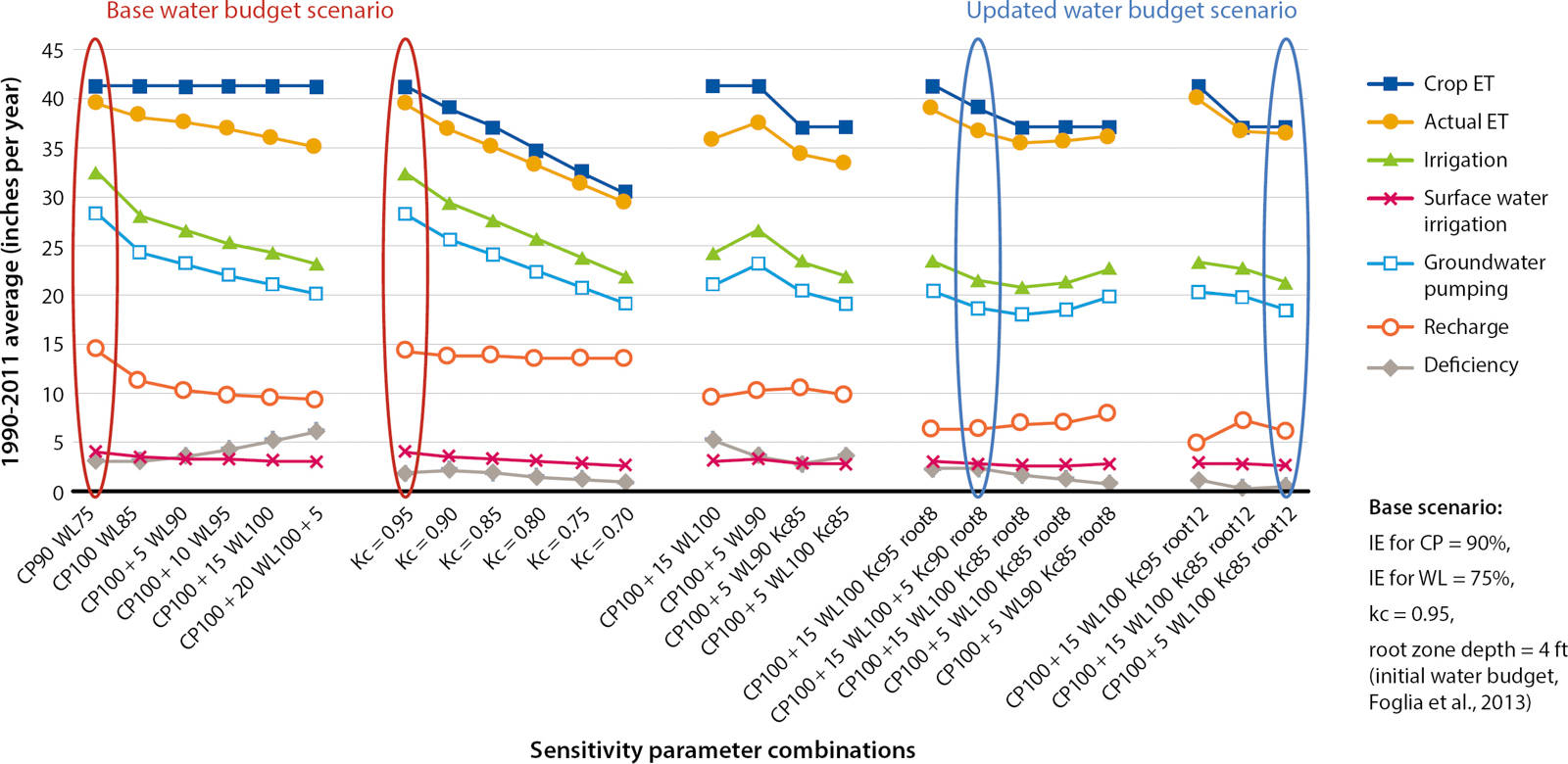
FIG. 4. Sensitivity of the simulated soil water fluxes to application efficiency, soil moisture depletion, root zone depth, and crop evapotranspiration (represented as crop coefficient Kc). For the soil water budget model sensitivity analysis, we adjusted root zone depth, from 4 feet (base value) to 8 feet (root8) and 12 feet (root12); alfalfa crop coefficient, from 0.95 (base value, Kc95) to 0.7; application efficiency for center-pivot from 90% (base value, CP90) to 100% + 20% SMDF (CP100 + 20), and for wheel-line from 75% (base value, WL75) to 100% + 5% SMDF (WL100 + 5); and (for deficit irrigation) the soil moisture depletion fraction (SMDF).
The scenarios offered several combinations of these parameters that resulted in irrigation amounts of 24 inches or less: Reducing the Kc value led to lower irrigation needs but conflicted with previously measured Kc values (0.95). Increasing application efficiency, increasing the soil moisture depletion fraction for deficit irrigation and increasing root zone depth all led to significant reductions in simulated irrigation without significantly affecting simulated evapotranspiration. It remained unclear which parameter option to choose.
A 3-year field research project was launched in cooperation with local growers to measure evapotranspiration, irrigation water applications and deep soil moisture profiles in eight alfalfa fields distributed across representative locations in Scott Valley. The study established a new, slightly lower Kc value of 0.9. For alfalfa, the soil water profile from 5 feet to 8 feet was found to generally decline in soil water content throughout the irrigation season. Thus, alfalfa was found to be effectively deficit irrigated, that is, the application efficiency was 100%. Experimental results better constrained input choices in SWBM. Using an 8-foot root zone for alfalfa, the new Kc = 0.9 value and soil moisture depletion fractions of 5% for wheel-line irrigation and 15% for center-pivot irrigation (on both alfalfa and grain), the total annual simulated irrigation depth on alfalfa, computed by the adjusted SWBM, averaged 22 inches per year instead of 33 inches per year, corresponding with measured irrigation rates (blue oval in fig. 4).
Aggregated water budget results from this calibrated SWBM provided some important insights into understanding the groundwater–surface water interface dynamics (table 1): The total amount of groundwater pumping (an output from the groundwater account) was equal to about two-thirds of the estimated total landscape recharge (an input to the groundwater account). Since long-term groundwater levels were balanced, the surplus in recharge relative to pumping, 14,000 acre-feet per year, was the net contribution of the landscape to base flow, that is, to the groundwater discharge to the Scott River.

TABLE 1. Aggregated average annual water budget model results over the 21-year simulation period by land use
A small portion of the 14,000 acre-feet per year may also contribute to evapotranspiration from ground-water (e.g., riparian vegetation). Note that actual net groundwater discharge to the Scott River is higher, as SWBM does not account for about 44,000 acre-feet per year of mountain-front recharge from tributaries and leakage to groundwater from irrigation ditches (a result obtained from the groundwater–surface water modeling, below). The total amount of net groundwater discharge to streams is only about one-tenth of the much larger Scott River total annual flow, most of which originates from the upper watershed. However, during the low flow period (July/August through September/October) the Scott River outflow from the basin is mostly groundwater dependent, particularly in dry years. Over that period, total stream outflow from the valley may amount to less than 10,000 acre-feet, and in exceptionally dry years (e.g., 2001, 2014, 2015) to less than 2,000 acre-feet. Relative to these flows, landscape recharge contribution to base flow was significant.
SWBM did not account for recharge contributions to groundwater from streams or for the dynamics of groundwater discharge to streams. SWBM also did not provide insight in how those may be affected by groundwater pumping and recharge or by intentional groundwater storage in the basin (a potential future project). For these additional analyses, SWBM must be coupled to a more complex groundwater–surface water model.
Importantly, SWBM was an important tool for outreach and education. That outreach led to initiation of the new field research, results from which improved model development. Refinement of SWBM was made possible through regular interactions between local stakeholders and growers on the groundwater advisory committee, the local UCCE farm advisor, the modeling team and the new field research. The collaboration on the SWBM increased the community's trust of the groundwater–surface water (MODFLOW) model component of SVIHM. (SWBM drives the pumping and recharge condition in the MODFLOW component, which in turn drives the dynamics at the groundwater–surface water interface.)
Water fluxes: RIV versus SFR representations
The groundwater–surface water model component of SVIHM, represented using both the RIV and SFR packages, simulated 21 years of groundwater and stream flow dynamics driven by monthly data of the statistically simulated stream inflows at each tributary from the upper watershed, by pumping in nearly 200 wells and by recharge from over 2,000 land parcels. Output included monthly water levels, groundwater flow directions and amounts, and groundwater–surface water exchanges at the 50-meter scale throughout Scott Valley for water years 1991 to 2011 (fig. 5).
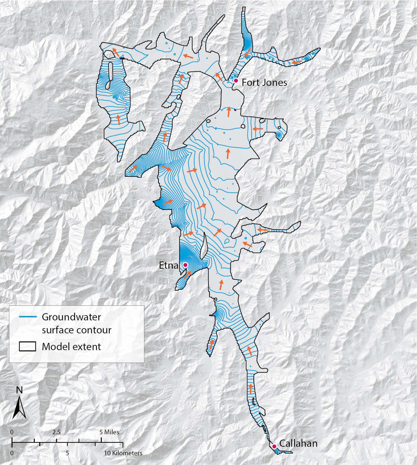
FIG. 5. Groundwater levels and flow direction in August 2001. This is one of the results from the groundwater–surface water model. Other output from the groundwater–surface water model included monthly water levels, groundwater flow directions and amounts, and groundwater–surface water exchanges for water years 1991 to 2011. Arrows indicate the flow direction but are not scaled to groundwater flow velocity. See supporting information S1 for comparison of simulated water levels and flow rates to measured water levels and flow rates. Source: Model extent derived from Mack (1958) and SSURGO data. Projection: North American Datum 1983, UTM Zone 10.
Sensitivity analysis and calibration of the numerical MODFLOW-based groundwater–surface water simulation model were completed to assess model performances and to fine-tune model parameters ( supporting information S1 and Tolley et al., unpublished data). These steps were taken to ensure that SVIHM's input and structure yielded simulation results that were consistent with 1991 to 2011 measured water level and long-term stream gauging information on the Scott River.
Groundwater budgets, including groundwater–surface water fluxes, will be one of the critical components evaluated and discussed by groundwater sustainability agencies. It's important to understand how to read the groundwater budget outputs from the conceptually very different RIV and SFR models and how the difference in the model can affect predictions of future scenarios.
SVIHM-RIV and SVIHM-SFR fundamentally differ in the representation of the elevation of the stream's water surface (stream state) — one user defined, one based on a streamflow model. In all other aspects, they are identical. The RIV representation, which lets the user specify stream stage (water level elevation) at each river cell, is an excellent option where water depth in the stream does not vary significantly in time or measurements are available about changes in stream stage at high spatial resolution and where these are not impacted or impacted in known ways under future scenarios of interest. Our very simplified RIV representation (constant, uniform stream water depth) was developed as a simplified conceptual approach to generate a first-order approximation of the groundwater–surface water interface, and we had no stream depth data.
In contrast, in the SFR representation, stream stage is simulated by a stream flow routing model that internally computes stream water levels while preserving water balance within the stream system dynamically. Stream stage at each grid cell is a function of stream flow into the cell, of physical characteristics of the stream available from detailed surveys and of groundwater–surface water fluxes at each grid cell. The SFR representation also accounts for the confluence of streams and for diversions to surface water users, which in turn affect local stream flow rates. When flow is insufficient to support stream flow, the streambed falls dry until either upstream inflow becomes available or groundwater begins to emerge into the streambed due to a higher water table. Given data available for Scott Valley and the dynamics of its stream system, MODFLOW SFR provided a physically more accurate, if computationally more expensive, model representation.
Aquifer water budgets for both the irrigation season (summer) and the nonirrigation season (winter) (fig. 6) showed that exchange of water between surface water and groundwater was about three times larger in SVIHM-RIV than SVIMH-SFR. All other boundary fluxes were identical due to both models having otherwise identical boundary conditions. In figure 6, the exchange between surface water and groundwater is represented in green and labeled “Stream”. For all the terms in figure 6, the flow “in” represents the amount of water entering into the aquifer from various sources, while the flow “out” is the flow leaving the aquifer.
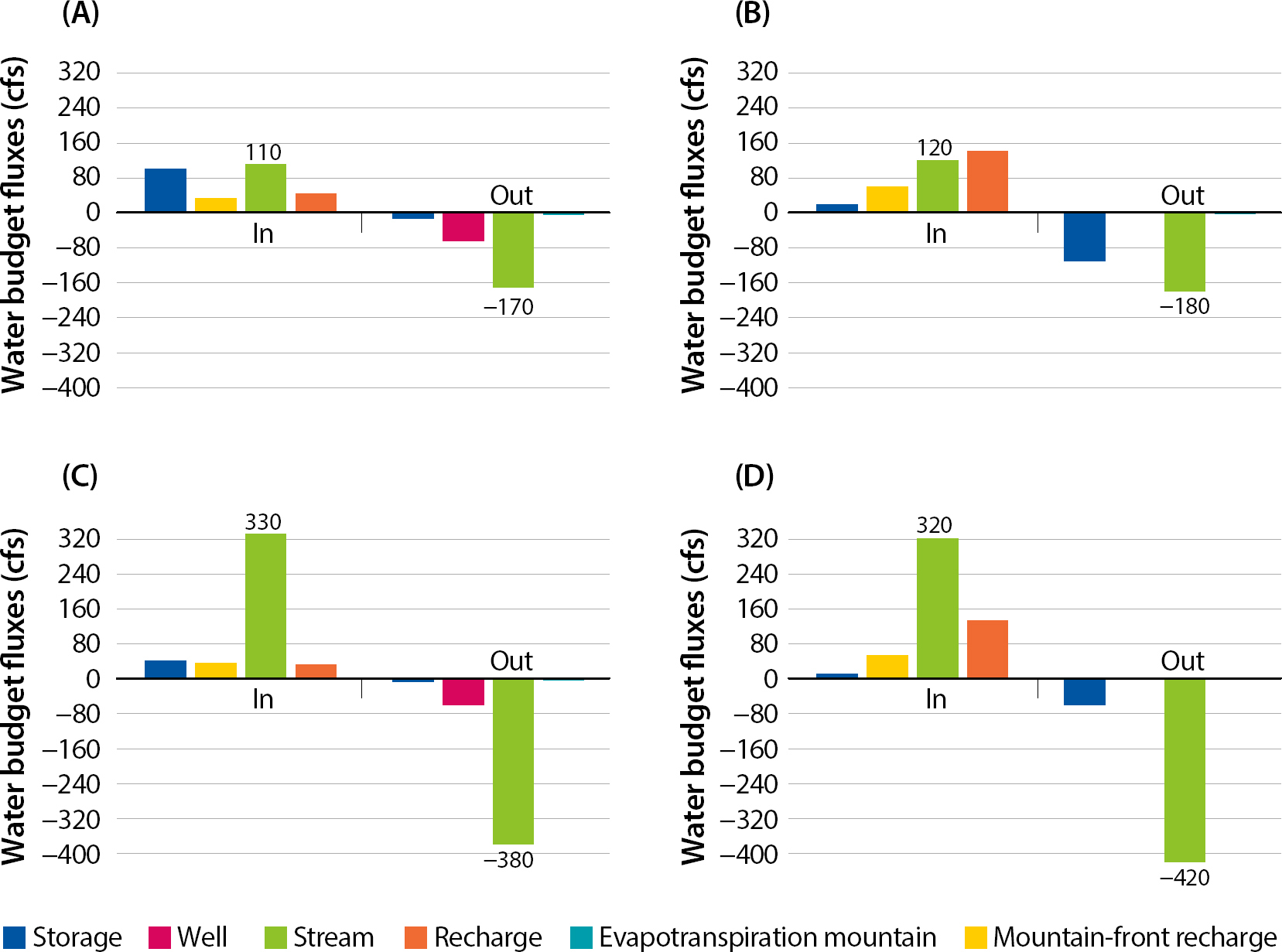
FIG. 6. Water budget results for various seasons and stream models. Markedly different groundwater–surface water fluxes were evident in the results of SFR and RIV models: (A) SFR during summer (the irrigation season, April to Sept), (B) SFR during winter (the nonirrigation season, October to March), (C) RIV during summer and (D) RIV during winter.
The difference between stream recharge (input to the water budget) and groundwater discharge (output from the budget), however, is the same in both models — a net groundwater discharge to the stream of 80 cfs (58,000 acre-feet per year), when averaged over the entire year. This is not coincidental: The net groundwater discharge of 58,000 acre-feet per year is independent from the groundwater–stream connectivity. It is instead entirely driven by the average annual difference between mountain-front recharge (determined by the upper watershed model), ditch losses to groundwater (user input based on measured data) and landscape recharge (SWBM result) on the one hand and ground-water pumping (SWBM result) and evapotranspiration losses from groundwater (MODFLOW result) on the other hand, none of which is a function of the choice of RIV or SFR package. The exception was the MODFLOW simulated evapotranspiration losses from groundwater near streams, which may be affected by the model choice (RIV or SFR).
With SVIHM-SFR, net groundwater discharge (fig. 6, difference between the Stream “in” and the Stream “out”) was only slightly smaller over the summer months than over the winter months (about 60 cfs in both seasons). In contrast, with SVIHM-RIV, the net discharge to streams was about 50 cfs in summer but almost 140 cfs in winter. This large seasonal variation was driven by seasonal variations in groundwater storage that operate differently in the SVIHM-RIV model than in the SVIHM-SFR model: Groundwater storage during winter increased in SVIHM-RIV by just 40 cfs, or 15,000 acre-feet per 6 months, half the increase in SVIHM-SFR (80 cfs, or 29,000 acre-feet per 6 months), due to the larger winter net groundwater-to-stream discharge in SVIHM-RIV. By the same token, groundwater storage during summer decreased in SVIHM-RIV by just half of that in SVIHM-SFR due to the much lower net groundwater-to-stream discharge in SVIHM-RIV in summer.
The difference between the simulated fluxes was caused by differences in the stream stage between SVIHM-RIV and SVIHM-SFR. The SVIHM-SFR model relied on measured and estimated stream flow entering the valley, which in turn drove the local and seasonal dynamics of stream stage and the magnitude of groundwater–surface water interaction. Inflows to the valley are highly dynamic and vary strongly between winter and summer. The SVIHM-RIV model with its uniform, constant stream water depth that we chose did not sufficiently capture the spatial and temporal changes in stream flow dynamics. In this simplified representation, the stream became an artificial buffer to groundwater level changes. SVIHM-RIV added recharge from streams during the low flow periods when no exchange occurred in SVIHM-SFR simulations.
When using SVIHM-RIV, it would therefore be important that dry stream sections are properly characterized a priori for simulating future management projects. Also, even in flowing sections of the stream, characterization could be improved by providing spatially more detailed, seasonally varying water level depth within the stream network as part of the RIV representation. In Scott Valley, however, one of the future scenario modeling goals for which the model will be used is to predict the change in the timing and extent of dry stream sections in response to groundwater management actions. For that purpose, only the SVIHM-SFR approach can be used.
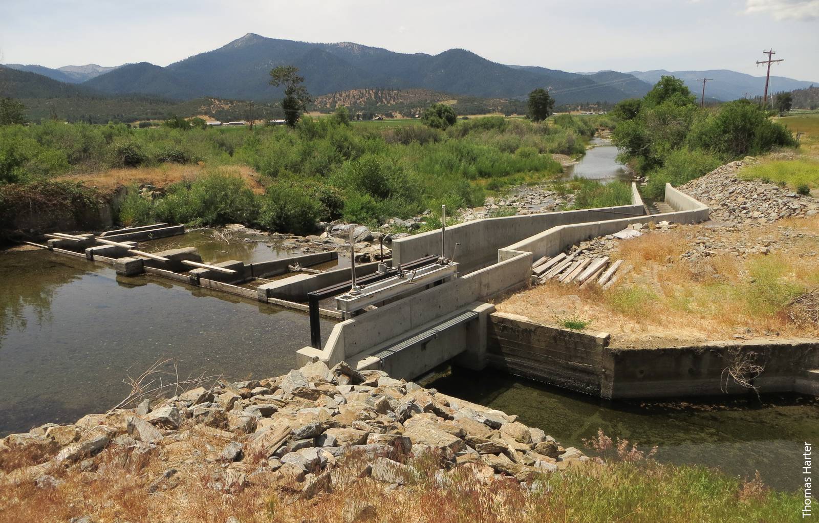
Scott Valley Irrigation District diversion and fish ladder. The river and its tributaries are an important salmonid spawning habitat, home to native populations of the threatened Oncorhynchus kisutch (coho).
Our Scott Valley study suggests that knowledge of stream stage at high spatial and temporal detail is critical when representing the groundwater–surface water boundary with a RIV approach. More detailed calibration that has been carried out for the SVIHM-SFR model (Tolley et al., unpublished data) demonstrated that the presence of river reaches that become dry during a certain time in the summer was a critical observation to calibrate or validate SVIHM-SFR.
Models for SGMA implementation
Under California's new groundwater governance, groundwater sustainability agencies across the state have to consider the potential impact of new groundwater management measures on groundwater–surface water interaction and specifically on estimating the effect of groundwater management on surface water depletion. Only a groundwater model that also has some representation of streams can provide the spatially and temporally more detailed information on groundwater–surface water exchange that may be required when evaluating individual groundwater management projects and their impacts to stream flow.
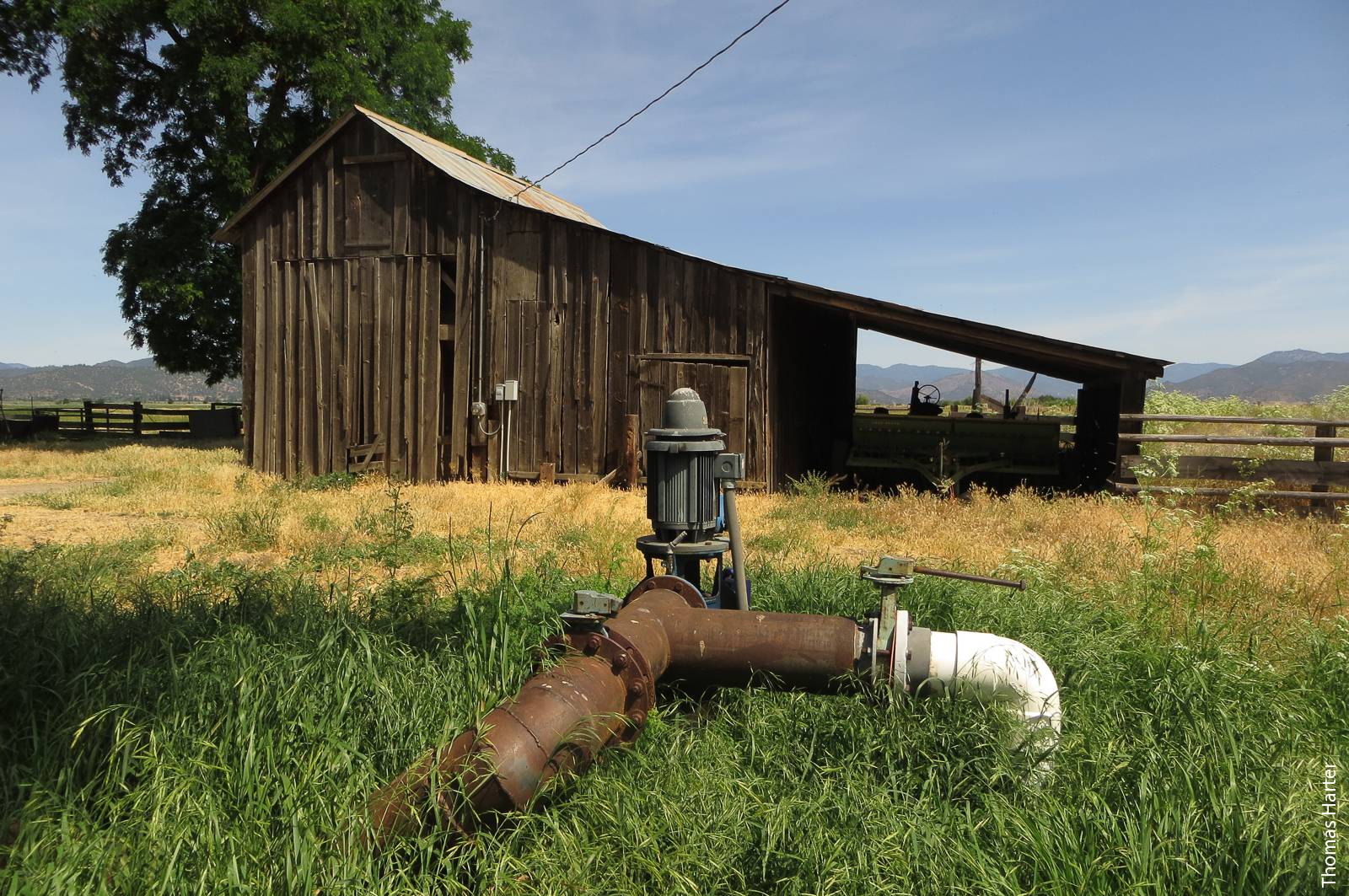
Irrigation well in Scott Valley.
As shown in our Scott Valley study, the choice of stream representation will depend on availability of data, data density in space, and data continuity in time for stream flow and stream stage. Depending on implementation, significantly different results may be obtained. The value of the model outcome will increase with better physical representation of the integrated hydrologic system, which in turn is driven by good data availability.
Integrated numerical modeling tools represent and link upper watersheds, the basin soil–landscape systems, the groundwater system and the basin surface water system. These tools will be useful to evaluate groundwater conditions (in SGMA referred to as sustainability indicators) and the benefits of management actions to address undesirable results. Some of these conditions, such as depletion of surface water by groundwater pumping, are otherwise difficult to measure from field data alone.
For the broader audience among groundwater agency stakeholder groups, the important take-away from our work is that numerical groundwater modeling tools are all based on the same mathematical representation of groundwater flow. But other elements of the hydrologic cycle to which a groundwater model must inevitably be linked — for example, the soil–landscape system, including the ways in which urban and agricultural water demands operate; the stream system; and the upper watershed system — are subject to more varied model representations. This variability affects the simulation of groundwater–surface water interface, pumping, recharge from various sources, and flows of surface water and groundwater at the basin boundaries.
As we demonstrated, an integrated model is not only a platform for a unifying, scientifically defensible framework to connect spatially and temporally distributed data of many different kinds and to represent a range of groundwater (and surface water) sustainability indicators. It is also a tool to explore conceptual uncertainties and initiate additional research and data collection to improve representation of the driving elements of groundwater–surface water interactions and other drivers of groundwater dynamics. The integration of various model components also (1) allows representation of fluxes within the basin and between different basins, (2) allows evaluation of the sensitivity of the integrated model to different parameters and observations, (3) facilitates an estimate of the uncertainty in the results (Tolley et al., unpublished data) and (4) supports the design of future management scenarios (not yet implemented here).
Our Scott Valley study shows that models of various complexity (regression model, mass balance model, and numerical dynamic model) can be successfully integrated and provide a useful interface to communicate with and successfully engage stakeholders in developing groundwater sustainability plans. Our results demonstrate the importance for stakeholders to fully understand the conceptual implications of the different assumptions of model development and how these can impact water budgets and management of fluxes between basins. This understanding is fundamental for the successful development of groundwater sustainability plans as required by SGMA.
Modeling guides groundwater management in a basin with river–aquifer interactions