


All Issues
Field procedure helps calculate irrigation time for cracking clay soils
Publication Information
California Agriculture 48(4):33-36.
Published July 01, 1994
PDF | Citation | Permissions
Abstract
Available soil moisture and low soil salinity are difficult to maintain in clay soils of arid regions due to the clay's low permeability. However, a simple procedure has been developed for estimating the duration of flood irrigation needed to saturate the cracked profile in these soils, while improving water conservation through limiting excess runoff. Using a worksheet, the irrigator makes a few measurements, then calculates how long to irrigate each border.
Full text
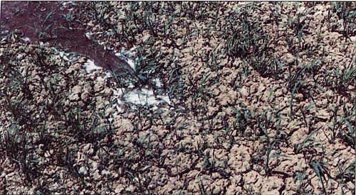
Cracking clay soils are common to many arid regions of the world, including some of the western states. In California these soils are found on the west side of the San Joaquin Valley, and also in the Imperial Valley, where silty clays comprises over 40% of the irrigated soils. Profitable crop cultivation on these heavy saline soils depends on controlling soil moisture conditions to maintain adequate infiltration and salt leaching of the root zone. Cracks may serve as conduits into these soils for adequate amounts of water to wet and leach the soil profile. This study focused on water conservation and irrigation management.
Our goal was to develop a simple procedure for use in the field that would tell the irrigator when to cut off border-check irrigation of cracking clay soils so that infiltration is maximized and runoff (tailwater) is minimized. The procedure we worked out has been used successfully in a field in the Imperial Valley. The irrigator takes a few simple measurements and does a brief set of calculations on a worksheet, all in the field.
Border-irrigation modeling
The procedure is based on the volume balance model for surface irrigation and the observation that cracking clay soils tend to allow infiltration of a constant volume of water per unit length of border, depending on crack volume. In fact, the crack volume of the field can be estimated from the proposed procedure. This volume increases as the soil profile dries.
As water advances along a border check, some moves along the surface and the rest infiltrates the soil. In cracking clay, after initial wetting there is often negligible infiltration into the clay component of the soil because of its very low permeability; instead, the advancing water primarily fills the soil cracks.
The volume balance model is a simple expression equating the sum of the surface water (SW) and the infiltrated water (IW) volumes to the total applied water (TAW) volume. Assuming a constant volume of infiltration per unit length of border and a constant onflow rate, the volume balance may be written:
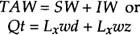
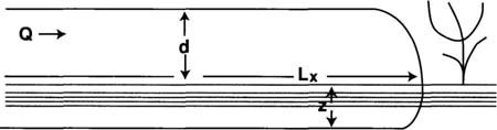
where Q is the average onflow rate (cfs) up to time t (sec), Lx is the advance distance of the surface-wetting front (ft) at time t, w is the border width (ft), d is the surface flow depth (ft) and z is the infiltrated water depth (ft). Figure 1 schematically illustrates in a cross-sectional view the different terms of the volume balance equation. In the model we assume that the cracks provide the only infiltration capacity; that is, there is a constant volume of cracks to fill every foot distance down the border. We cannot generally make such an assumption for noncracking soils. All of the equation parameters are easily measured, except for d and z. The infiltration depth, z, is rarely measured directly; instead, it is determined from the volume balance equation after the other parameters have been measured.
The flow depth, d, though simple in concept, is often multiplied by a “shape factor” to account for variations in soil surface microtopography and the shape of the water surface profile. Although the shape factor can be ignored when Lx is large relative to d, variable microtopography still makes accurate measurement of flow depth difficult in the field. For example, we directly measured flow depth with two different sets of 10 depth-gauges during three irrigation events and found the effort labor intensive and highly variable (the standard deviation in the measurements was 60 to 77% of the average or mean value). The direct measurements also resulted in poor prediction of irrigation cutoff times.
As an alternative to direct measurements, we estimated average flow depth from a variation of Manning's equation for shallow flow in wide open channels. Manning's equation is a widely used, semiempirical equation developed by hydraulic engineers in the last century; it relates flow depth, channel slope, surface roughness and flow rate. For a wide channel with shallow flow depth relative to the width of the channel, Manning's equation may be written as:
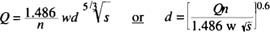
where n is the surface roughness, s is the surface slope (ft/ft) and the other parameters are as previously defined.
In practice, the surface slope of the field is commonly known (having been measured when the field was initially graded); however, the value of the surface roughness coefficient, n, must be estimated independently. Values of n will vary with cultivation practice, the particular crop and the stage of crop growth. We found that the value of n increases from approximately 0.011 for the first irrigation of a newly cultivated and seeded field to approximately 0.015 for the next irrigation at plant emergence, to roughly 0.027 for forage crops (cereal grains, Sudan grass) nearing maturity.
Estimating cutoff times
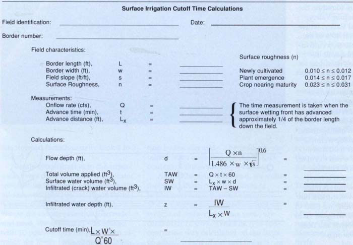
The worksheet outlining the calculations necessary to determine the irrigation cutoff time is shown in table 1. The information required to complete the worksheet includes the field characteristics (such as border width) and measurements taken during the irrigation (such as onflow rate). For many fields, most of the field data (Q, w, s and L) change little during the irrigation season, so that relatively little time or effort is needed to update the worksheet as the season progresses.
Border-irrigated fields are often 1/4 or 1/2 mile long and have a very gradual slope, minimal cross-slope and variably spaced border checks. Our study was of 1/4-mile border lengths, though the concepts also apply to borders of longer lengths. The recommended field slopes for border-irrigated fields are less than 0.01 ft/ft (1%), with a minimum of approximately 0.001 ft/ft (0.1%). The cross-slope should be less than 0.1% to minimize uneven spreading of water between border checks. Border width depends on the cultural practices for the crop, the available onflow rate and the slope of the field. Border-check spacings of roughly 30 ft for field slopes on the order of a few tenths of a percent and 60 ft for relatively flat slopes are common. In the Tulare Basin, border widths are often several hundred feet because of the flat topography and the capacity to deliver large flow rates to the field. Sometimes, the first 30 to 40 ft at the head end of the field is graded flat to facilitate spreading of applied water across the full width of the border before it begins moving down the border. Thus, for a typical small field in the San Joaquin or Imperial valleys, values of L = 1,300 ft, w = 50 ft, and s = 0.002 ft/ft may be appropriate.
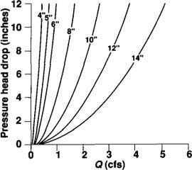
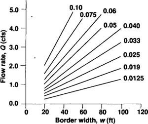
To apply the volume balance model, the irrigator must know the dimensions and slope of the borders before irrigating and then measure the onflow rate and the time required for the surface wetting front to reach approximately 1/4 the length of the border (e.g., 330 ft for a 1,300-ft border) during the irrigation. The border dimensions and slope are measured during field preparation, and the surface roughness is estimated from the ranges given in the worksheet. The onflow rate can be measured directly in the delivery pipe with a flow meter if alfalfa valves are used, or by measuring the pressure head drop across an irrigation turnout (spile) in conjunction with a calibration table or graph (fig. 2) if turnouts or large siphons are used. The pressure head drop is equivalent to the difference in water surface elevations between the head ditch and the field; it can be measured with a transit, a hand level or a manometer tube across the turnout together with a yardstick. Once the pressure head drop is known, the onflow rate can be estimated from figure 2 by entering the graph through the value of the pressure head drop on the vertical axis moving horizontally across to the curve corresponding to the turnout size and vertically down from the point of intersection on the curve to the horizontal axis displaying the flow rate. For example, a pressure head drop of 5 inches across a 10-inch-diameter turnout yields an onflow rate of 1.70 cfs per turnout or siphon.
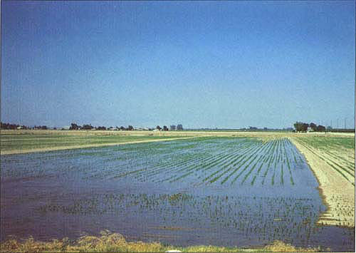
In the field, an irrigator can take a few measurements then calculate when to cut off border-check irrigation of cracking clay soils to maximize infiltration and minimize runoff.
After irrigation begins, the irrigator should note the time required for the average position of the surface wetting front to reach markers placed in the border checks approximately 1/4 the length of the border, then calculate the cutoff time using the worksheet. Most of the calculations require simple multiplication, division, addition or subtraction; the exception is flow depth.
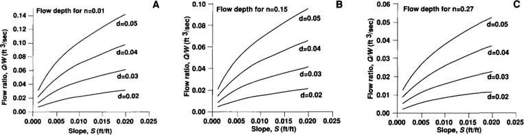
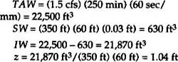
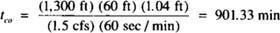
To simplify determination of flow depth, we prepared a graphical calculation of flow depth (fig. 3 and fig. 4). With knowledge of Q (onflow rate) and w (border width), the flow/width ratio, Q/w, can be determined from figure 3 (or it can be calculated directly for flow rates and border widths greater than those given in the figure, such as those in the Tulare Basin). For example, an onflow rate of 1.5 cfs on a border 60 ft wide has a flow/width ratio of 1.5/60 = 0.025. With knowledge of the flow/width ratio, the slope of the field and an estimate of the surface roughness, the flow depth can be estimated using the appropriate graph in figure 4. Continuing with the example above, for a flow/width ratio of 0.025, a field slope of 0.008 ft/ft and a surface roughness of n = 0.015, the flow depth is 0.03 ft (from fig. 4b). This result can now be substituted into the worksheet and the remaining calculations completed. If the irrigator measured an advance time of 250 min for the wetting front to reach 350 ft down a field 1,300 ft long, then from the worksheet in table 1, and the cutoff time for this field is or 15 hours of total irrigation time.
The crack volume of a field can be estimated from the volume balance model.
If the onflow rate, field dimensions and slope are unchanged from one irrigation to the next, then the time required for the surface wetting front to reach the markers will increase somewhat as the crop matures and the surface roughness increases and the soil becomes progressively drier resulting in greater crack volume (though this time required for the advance will vary with the irrigation schedule adopted). After several irrigations, the worksheet may not be needed, because the irrigator will have become familiar with the time required to leave the turnouts open in order to irrigate the particular field satisfactorily.
Results from field studies
We applied this procedure for calculating cutoff times to the border-irrigated clay field in the Imperial Valley considered in previous California Agriculture reports (November-December 1990, September-October 1992). The field is 1/4 mile long and has 60-ft-wide borders on a small slope of roughly 0.1%; each border check is irrigated from a 12-inch-diameter turnout at the head ditch. The turnouts for this field had been calibrated earlier by Tod et al. (ASCE Journal of Irrigation & Drainage Engineering 117(4): 596–599, 1991), and the measured calibration curve was similar to that given in figure 2. Individual borders were planted with alfalfa, barley and Sudan grass.
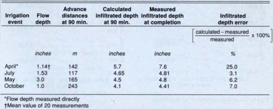
Table 2 summarizes results from four different irrigations for which we calculated cutoff times. For the April irrigation, we measured the flow depth using the depth-guages described earlier; for the remaining three irrigations, we estimated flow depth from Manning's equation. For the April irrigation, we underestimated the cutoff time, and the border was incompletely irrigated; in the remaining irrigations, the border was completely irrigated with little or no measurable tailwater runoff. We had errors of 3 to 7% in the infiltrated depths, which are consistent with the errors associated with the roughness coefficient, n, and the various measurement errors encountered with field measurements of flow rate, slope and advance time. From these and similar observations, we are developing rule-of-thumb estimates of irrigation times for this clay field. We are also using this procedure to estimate crack volumes in the field so as to devise better irrigation-drainage management strategies for clay soils.
Field procedure helps calculate irrigation time for cracking clay soils