Day 3: I opened the day with a lovely swim with Elizabeth Havice (in the largest pool in New England? Boston? The Sheraton?) and then embarked on a multi-mile walk around the fair city of Boston. The sun was out and the wind was up, showing the historical buildings and waterfront to great advantage. The 10-year old Institute of Contemporary Art was showing in a constrained space, but it did host an incredibly moving video installation from Steve McQueen (Director of 12 Years a Slave) called “Ashes” about the life and death of a young fisherman in Grenada.
My final AAG attendance involved two plenaries hosted by the Remote Sensing Specialty Group and the GIS Specialty Group, who in their wisdom, decided to host plenaries by two absolute legends in our field – Art Getis and John Jensen – at the same time. #battleofthetitans. #gisvsremotesensing. So, I tried to get what I could from both talks. I started with the Waldo Tobler Lecture given by Art Getis: The Big Data Trap: GIS and Spatial Analysis. Compelling title! His perspective as a spatial statistician on the big data phenomena is a useful one. He talks about how data are growing fast: Every minute – 98K tweets; 700K FB updates; 700K Google searches; 168+M emails sent; 1,820 TB of data created. Big data is growing in spatial work; new analytical tools are being developed, data sets are generated, and repositories are growing and becoming more numerous. But, there is a trap. And here is it. The trap of Big Data:
10 Erroneous assumptions to be wary of:
- More data are better
- Correlation = causation
- Gotta get on the bandwagon
- I have an impeccable source
- I have really good software
- I am good a creating clever illustrations
- I have taken requisite spatial data analysis courses
- It’s the scientific future
- Accessibly makes it ethical
- There is no need to sample
He then asked: what is the role of spatial scientists in the big data revolution? He says our role is to find relationships in a spatial setting; to develop technologies or methods; to create models and use simulation experiments; to develop hypotheses; to develop visualizations and to connect theory to process.
The summary from his talk is this: Start with a question; Differentiate excitement from usefulness; Appropriate scale is mandatory; and Remember more may or may not be better.
When Dr Getis finished I made a quick run down the hall to hear the end of the living legend John Jensen’s talk on drones. This man literally wrote the book on remote sensing, and he is the consummate teacher – always eager to teach and extend his excitement to a crowded room of learners. His talk was entitled Personal and Commercial Unmanned Aerial Systems (UAS) Remote Sensing and their Significance for Geographic Research. He presented a practicum about UAV hardware, software, cameras, applications, and regulations. His excitement about the subject was obvious, and at parts of his talk he did a call and response with the crowd. I came in as he was beginning his discussion on cameras, and he also discussed practical experience with flight planning, data capture, and highlighted the importance of obstacle avoidance and videography in the future. Interestingly, he has added movement to his “elements of image interpretation”. Neat. He says drones are going to be routinely part of everyday geographic field research.
What a great conference, and I feel honored to have been part of it.
Between the years 1949-1979 the Pacific Southwest research station branch of the U.S. Forest service published two series of maps: 1) The Soil-Vegetation Maps, and 2) Timber Stand Vegetation Maps. These maps to our knowledge have not been digitized, and exist in paper form in university library collections, including the UC Berkeley Koshland BioScience Library.
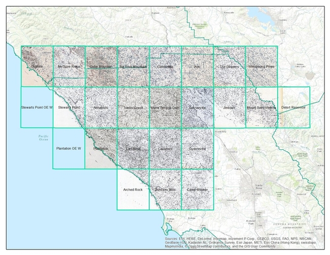
Index map for the Soil Vegetation MapsThe Soil-Vegetation Maps use blue or black symbols to show the species composition of woody vegetation, series and phases of soil types, and the site-quality class of timber. A separate legend entitled “Legends and Supplemental Information to Accompany Soil-Vegetation Maps of California” allow for the interpretation of these symbols in maps published 1963 or earlier. Maps released following 1963 are usually accompanied by a report including legends, or a set of “Tables”. These maps are published on USGS quadrangles at two scales 1:31,680 and 1:24,000. Each 1:24,000 sheet represents about 36,000 acres.
The Timber Stand Vegetation Maps use blue or black symbols to show broad vegetation types and the density of woody vegetation, age-size, structure, and density of conifer timber stands and other information about the land and vegetation resources is captured. The accompanying “Legends and Supplemental Information to Accompany Timber Stand-Vegetation Cover Maps of California” allows for interpretation of those symbols. Unlike the Soil-Vegetation Maps a single issue of the legend is sufficient for interpretation.
We found 22 quad sheets for Sonoma County in the Koshland BioScience Library at UC Berkeley, and embarked upon a test digitization project.
Scanning. Using a large format scanner at UC Berkeley’s Earth Science and Map library we scanned each original quad at a standard 300dpi resolution. The staff at the Earth Science Library completes the scans and provides an online portal with which to download.
Georeferencing. Georeferencing of the maps was done in ArcGIS Desktop using the georeferencing toolbar. For the Sonoma county quads which are at a standard 1:24,000 scale we were able to employ the use of the USGS 24k quad index file for corner reference points to manually georeference each quad.
Error estimation. The georeferencing process of historical datasets produces error. We capture the error created through this process through the root mean squared error (RMSE). The min value from these 22 quads is 4.9, the max value is 15.6 and the mean is 9.9. This information must be captured before the image is registered. See Table 1 below for individual RMSE scores for all 22 quads.
Conclusions. Super fun exercise, and we look forward to hearing about how these maps are used. Personally, I love working with old maps, and bringing them into modern data analysis. Just checking out the old and the new can show change, as in this snap from what is now Lake Sonoma, but was the Sonoma River in the 1930s.

Thanks Kelly and Shane for your work on this!
I wanted to send out a friendly reminder that the data submission deadline for the current data call is March 31, 2016. Data submitted before March 31 are evaluated for inclusion in the appropriate update cycle, and submissions after March 31 are typically considered in subsequent updates.
This is the last call for vegetation/fuel plot data that can be used for the upcoming LANDFIRE Remap. If you have any plot data you would like to contribute please submit the data by March 31 in order to guarantee the data will be evaluated for inclusion in the LF2015 Remap. LANDFIRE is also accepting contributions of polygon data from 2015/2016 for disturbance and treatment activities. Please see the attached data call letter for more information.
Brenda Lundberg, Senior Scientist
Stinger Ghaffarian Technologies (SGT, Inc.)
Contractor to the U.S. Geological Survey (USGS)
Earth Resources Observation & Science (EROS) Center
Phone: 406.329.3405
Email: blundberg@usgs.gov
Developing data-driven solutions in the face of rapid global change
Global environmental change poses critical environmental and societal needs, and the next generation of students are part of the future solutions. This National Science Foundation Research Traineeship (NRT) in Data Science for the 21st Century prepares graduate students at the University of California Berkeley with the skills and knowledge needed to evaluate how rapid environmental change impacts human and natural systems and to develop and evaluate data-driven solutions in public policy, resource management, and environmental design that will mitigate negative effects on human well-being and the natural world. Trainees will research topics such as management of water resources, regional land use, and responses of agricultural systems to economic and climate change, and develop skills in data visualization, informatics, software development, and science communication.
In a final semester innovative team-based problem-solving course, trainees will collaborate with an external partner organization to tackle a challenge in global environmental change that includes a significant problem in data analysis and interpretation of impacts and solutions. This collaboration is a fundamental and distinguishing component of the NRT program. We hope this collaboration will not only advance progress on the grand challenges of national and global importance, but also be memorable and useful for the trainees, and for the partners.
An Invitation to Collaborate
We are inviting collaboration with external partners to work with our students on their Team Research Project in 2016-17. Our students would greatly benefit from working with research agencies, non-profits, and industry.
- Our first cohort of 14 students come from seven different schools across campus, each bringing new skillsets, backgrounds, and perspectives.
- Team projects will be designed and executed in the spring of 2017.
- Partners are welcome to visit campus, engage with students and take part in our project activities.
- Join us at our first annual symposium on May 6th 4-7 pm.
- Participate in workplace/ campus exchange.
- Contact the program coordinator at hconstable@berkeley.edu
- Visit us at http://ds421.berkeley.edu/ for more information.
This new NSF funded DS421 program is in the first of 5 years. We look forward to building ongoing collaborations with partners and UC Berkeley.
Awesome new (ish?) R package from the gang over at rOpenSci
Tired of searching biodiversity occurance data through individual platforms? The "spocc" package comes to your rescue and allows for a streamlined workflow in the collection and mapping of species occurrence data from range of sites including: GBIF, iNaturalist, Ecoengine, AntWeb, eBird, and USGS's BISON.
There is a caveat however, since the sites use alot of the same repositories the authors of the package caution to check for dulicates. Regardless what a great way to simplify your workflow!
Find the package from CRAN: install.packages("spocc") and read more about it here!


